


Catalyst sintering detective: telling particle growth from migration and coalescence
Follow supported catalyst particles as they grow, move and merge. Compare Ostwald ripening with particle migration and coalescence, inspect the evidence, then test your interpretation in a five-round quiz.
Larger particles, different routes
Catalyst particles can become larger while their total number and available surface area decrease. The same change in mean diameter can arise through different routes: atoms leaving small particles and joining larger ones, or particles moving across a support and merging when they meet. Understanding the route matters when deciding what to follow in an in situ experiment.
AEML’s third research tool, Catalyst sintering detective, turns these mechanisms into a TEM-like movie. Follow individual particles, compare size distributions and surface-area changes, then use a short quiz to test which evidence supports your interpretation.
Open the sintering detective →
Follow the particles, then read the statistics
The two mechanisms leave different clues in the movie.
- Ostwald ripening (OR): atoms transfer from smaller particles to larger ones. Look for particles that shrink and disappear in place while their larger neighbours grow.
- Particle migration and coalescence (PMC): particles move across the support and merge when they meet. Follow the trajectories and the disappearance of the boundary between a pair of particles.
Both routes reduce particle number and can increase mean size, so those two statistics alone do not settle the question. The tool places the movie beside the size distribution, particle-count history and growth plot. The surface readout tracks a geometric proxy for the exposed metal area.
Turn on Show evidence to see recent trajectories in blue and particles that have just vanished in place marked in red. Pause the movie and move the time slider to compare the events with the changing statistics.
Zoom in to a single crystal
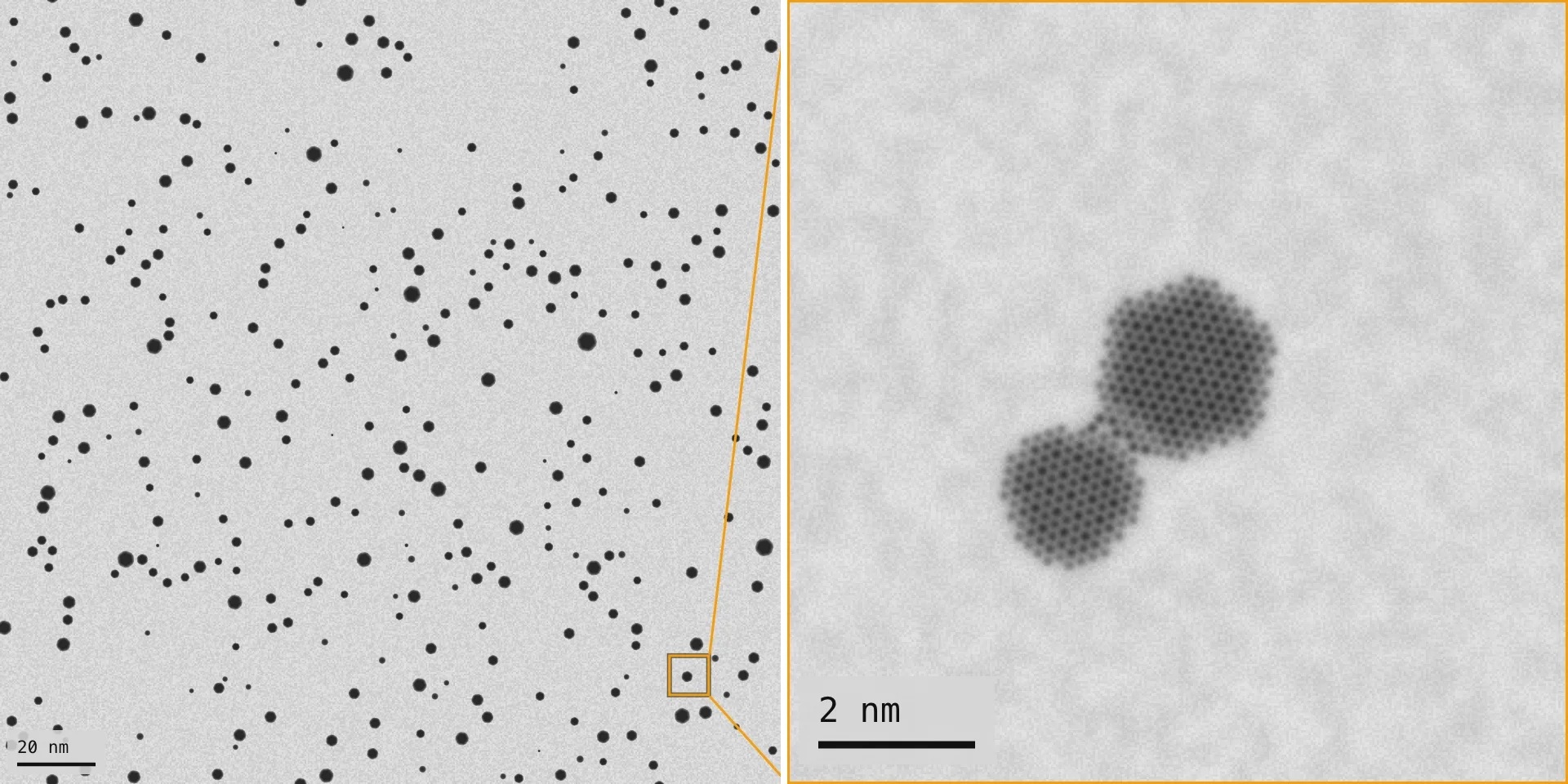
Below the movie, the Close-up view follows one event at a time: two particles about to merge, the merge itself or a particle about to vanish in place. The orange square in the movie shows where it is looking. Another scene moves to a different event, and clicking a particle in the movie follows that particle instead.
In a field only a few nanometres wide, an aberration-corrected microscope resolves the atomic columns of a Pt particle, so the close-up draws each particle as a crystal seen along the [111] zone axis. Each dot is a column of Pt atoms, 0.16 nm from its neighbours. Columns that hold more atoms appear brighter in HAADF and darker in bright field; the flat (111) top facet therefore looks even, while the {111} and {100} side facets fade towards the edge. When two crystals merge, the neck between them fills with the lattice of the particle that remains.
The particle shapes come from the Pt surface energies, and the columns count the atoms inside each shape. Every particle is assumed to sit on a (111) facet and so to lie on the zone axis, and bright field leaves out the focus- and thickness-dependent contrast of real lattice images. Necks and changes of shape are illustrations rather than part of the calculation. In a wide field that the screen cannot resolve at 0.16 nm, the close-up shows thickness contrast instead.
In the quiz, the close-up stays on the centre of the field and names no events until you answer. You can still click a particle to follow it.
Compare three example conditions
Start with Oxidizing gas: Ostwald ripening wins, Small particles, inert gas: migration wins and Both at once. These examples illustrate how the dominant contribution changes when the relative rates and initial particle sizes change.
Then adjust temperature, initial mean diameter, size spread and support coverage. The OR and PMC switches let you examine their separate contributions. Smaller particles move faster in the model, while changing the temperature rescales the rates through the selected activation energies. The oxidizing-gas example applies an illustrative acceleration to OR; its multiplier is not a universal property of oxidizing atmospheres.
The distribution view includes the LSW and Wagner reference curves for the modeled ripening regimes. Use them together with the movie: a distribution or a fitted growth exponent is one part of the evidence, and the individual particle events help explain it.
Test your interpretation with five hidden scenarios
Switch from Explore to Quiz. Each round shows a particle movie without revealing the selected mechanism. Decide whether the main process is OR, PMC or a combination of both, then check the explanation.
After you answer, the tool reveals the hidden scenario and evidence from the complete run: particles that vanished in place, merging events, the fraction of larger particles and the late growth exponent. The five-round sequence encourages you to compare what you saw with the evidence rather than relying on mean size alone.
The quiz is also useful in a group discussion. Pause at an event, ask what would need to be tracked in a real TEM series, and compare the reasons behind different answers.
Keep model time separate from experimental time
The model combines mean-field OR with Brownian particle migration on a two-dimensional support. Total particle volume is conserved, and merging follows contact. The TEM-like rendering provides a visual setting for these mechanisms; it is a simulation rather than an experimental micrograph.
The time axis is dimensionless model time. The rates and gas-response multiplier are illustrative, so the movie cannot be converted directly into a catalyst lifetime or a required heating duration. Likewise, the geometric surface-area proxy does not by itself predict catalytic activity.
Use Copy settings link to share a comparison. The inputs and random seed travel with the link, making the particle evolution reproducible for the same model version. The equations, assumptions and references are available below the interactive view.
How we built and checked the tool
We designed and implemented this tool with Claude Opus 5.5 Max in Claude Code. The starting question was whether watching individual particles could help distinguish the routes behind growth. We used the OR and PMC models to build the calculation module, particle movie, statistical plots and five-round quiz in TypeScript, React and Canvas.
The calculation code and tests were reviewed independently with Codex (GPT-6.1 Sol, Max), and the findings informed revisions. Checks covered total-volume conservation, the LSW and Wagner distributions and growth rates, and the mean-square displacement expected for Brownian migration. We also checked reproducibility with the same random seed, quiz scenarios and desktop and mobile interactions.
The single-crystal close-up was added later in the same way. It was designed and implemented with Claude Opus 5.5 Max in Claude Code, and the finished code was reviewed independently by a separate Claude Opus 5.5 reviewer and by Codex (GPT-6.1 Sol, Max). The checks compared the atoms in every column with a one-by-one count of the atoms in each shape and confirmed that the lattice follows the (111) orientation used in the nanoparticle shape tool. They also verified that quiz captions name no mechanism before an answer, that the same seed still reproduces the same run, and that playback holds 15 frames per second with 1,200 particles in a desktop browser.
Open the tool and try the five-round quiz →
To explore changes in the shape of one particle, see Gas-responsive nanoparticle shape. For acquisition timing and beam exposure, start with the Gas TEM planner.