


Gas TEM timing & dose planner: aligning gas changes with image acquisition
Compare gas arrival, image acquisition and beam blanking on one timeline. A practical guide to response calibration, incident fluence and sharing an experimental schedule.
Three timelines, one experiment
A Gas TEM experiment involves the gas-switch command, the changing environment at the specimen, and the periods when the electron beam is on. AEML’s Gas TEM timing & dose planner brings these together so that acquisition conditions can be compared before an experiment.
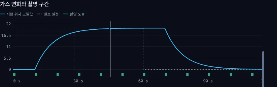
The gas-response plot shows the valve setting, modeled composition at the specimen and exposure windows. A second plot compares cumulative incident fluence under the selected imaging schedule with continuous illumination. Adjusting a parameter updates both plots, making it easier to ask: when should recording begin, how frequently should images be acquired, and what changes if the beam is blanked between frames?
Start with a comparison
The three example scenarios—Beam always on, Blank between frames and Short gas pulse—provide a starting point. Compare the gas trajectory, the acquisition windows and the cumulative fluence, then replace the example values with your planned conditions.
- Set the gas response. Enter the initial and target compositions, transport delay and mixing time constant. Choose a sustained change or a finite pulse.
- Set acquisition timing. Specify the observation duration, first exposure, exposure time and frame interval. The timeline shows how these windows overlap the modeled gas transition.
- Set the beam conditions. Enter incident current and the illuminated width and height, then compare continuous irradiation with blanking between frames.
The illuminated area is the area reached by the beam; it may differ from the camera field of view. The planner reports incident electrons per unit area, so this input matters when comparing schedules.
Replace the example response with measurements
The calibration section accepts the times at which a measured step response reaches 10% and 90% of its total change. It estimates a delay and mixing time constant for the planner’s simplified response model. Compare the result with the full measured trace before using it to choose acquisition timing.
An outlet measurement and the response at the specimen can have different delays. Calibration should reflect the observation conditions and measurement location; changes in flow, pressure or temperature may require a new response estimate.
Keep the conditions with the schedule
Use Copy settings link to create a link containing the current inputs. A collaborator can open it to review the same plan. Frame schedule CSV exports complete-frame start and end times, the modeled gas fraction averaged over each exposure, cumulative incident fluence and the input conditions. Calculations run in the browser.
The default conditions illustrate the comparison: 50 pA incident current, a 500 × 500 nm illuminated area, a 120 s observation window, and 1 s exposures every 10 s. This schedules 12 complete frames. With ideal blanking between frames, the calculated incident fluence is 90% lower than under continuous illumination over the same window. These are example calculations, not a measured reduction in specimen damage.
What the comparison means
The tool uses a delayed mixing model and assumes uniform rectangular illumination with ideal beam blanking. It helps compare timing and incident fluence under those assumptions. Material-specific reaction kinetics, adsorption, prior irradiation and beam-induced chemistry require experimental evidence beyond this model.
Use it to make acquisition choices explicit and record comparable conditions. The model assumptions and calculation details are available below the interactive plots.